Part V- Sampling and the Normal Distribution
Sample Sums, Sample Means, Sample Variances
Sample Mean and Variance as Estimators
The Variance of the Sample Average and Sample Sum
Standardizing a Random Variable
The Sample Average and Sum for a Normal Distribution
The Normal Approximation to the Binomial Distribution
Let F denote any given distribution. A random sample of size n from F is a sequence X1, X2, ..., Xn of random variables such that
1. X1, X2, ..., Xn are independent, and
2. The distribution of each individual variable Xi is the given distribution F.
In statistics it is usually assumed that the data at hand are values of a random sample from some distribution. The distribution F is usually unknown, at least partially, and the goal is to make inferences about it from the data.
The term "random sample" has a slightly different meaning here than it does when speaking of a random sample from a population.
The values of a random sample U1, U2, ..., Un from the standard uniform distribution on the interval (0, 1) may be simulated easily. Simply punch the random number key on your calculator n times. Once the values of U1, U2, ..., Un are simulated, the values of a random sample X1, X2, ..., Xn from the cumulative distribution function FX can be simulated by letting each Xi be the smallest solution x of the inequality Ui ≤ FX(x). For example, a random sample from the uniform distribution on the interval (a, b) can be obtained by letting Xi = a + (b-a)Ui.
Let X1, X2, ..., Xn be a random sample from a given distribution. Suppose this distribution has mean μ and variance σ2. From the random sample, we derive four new random variables of great imporance:

These are random variables. The last three should not be confused with the corresponding parameters μ, σ2 and σ, which are not random variables.
The sample sum, mean, variance and standard deviation are random variables and have distributions derived from the distribution sampled. As such, they have expected values. One of the most important properties of the sample mean and variance is that they are unbiased estimators of the corresponding population parameters μ and σ2. This means that

If the population mean and variance are unknown, they can be estimated from the data by the sample mean and variance. "On average" the estimated values will be right. The sample standard deviation is not, in general, an unbiased estimator of the population standard deviation. However, it is still useful as an estimator of the population standard deviation.
The expected value of a sum of random variables is the sum of their expected values. Thus, for the sample sum,
![]()
Because of the independence of the summands, the variances add in the same way.
![]()
It follows from the last equation that the variance of the sample average is

and its standard deviation is
![]()
The standard deviation of the sample sum is
![]()
If X is a random variable with mean μ and standard deviation σ, the standardized value of X is the random variable

The random variable Z is sometimes called the z-score of X. Its mean and variance are, respectively, 0 and 1. The standardized values of the sample sum and the sample average are algebraically equivalent because the sample sum is simply a multiple of the sample average. They are

For comparison, the standardized value of a binomial random variable Y based on n trials and success probability θ is

When the samples X1, ..., Xn are from a normal distribution with mean μ and standard deviation σ, the sample average and the sample sum are both normally distributed. The sample average has the normal distribution with mean μ and standard deviation σ/√n. The sample sum is normally distributed with mean nμ and standard deviation σ√n. Their standardized value has the standard normal distribution with mean 0 and standard deviation 1.
The sample average is normally distributed if the samples are from a normal distribution. The most important theorem in probability is the central limit theorem, which asserts that it is approximately normally distributed even when the samples are from a non-normal distribution, provided that the sample size is large enough. More precisely, as the sample size n gets large without bound, the distribution of the standardized sample average approaches the standard normal distribution. For any given numbers a and b, with a < b,

A binomial random variable is a sample sum Y = X1 + X2 + ... + Xn, where the Xi are independent Bernoulli trials. Therefore, the central limit theorem applies and for large enough n the distribution of the standardized value of Y

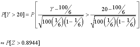
is approximately standard normal. As an illustration of how this might be useful, suppose a six-sided die is thrown 100 times and we want to know the probability that a 2 occurs more than 20 times. If Y is the number of occurrences of a 2 in the n=100 trials, we are after P[Y > 20]. The success probability θ is 1/6. With some algebra and the central limit theorem,

where Z has a standard normal distribution. From a table of the standard normal distribution we find that P[Z > 0.8944] = 0.1855. The exact value to four decimal places of the probability of more than 20 successes is 0.1519. One of the sources of inaccuracy is that we are trying to approximate a discrete distribution (the binomial) by a continuous distribution (the normal). The normal approximation can be improved by using what is known as the continuity correction. Observe that since Y is a whole number, the events [Y > 20] and [Y > 20.5] are the same. Replacing 20 by 20.5 in the calculations above results in an approximate value of P[Z > 1.0286] = 0.1518.