Random Walk

This script uses the function randomWalk to plot and display some statistics.

Contents

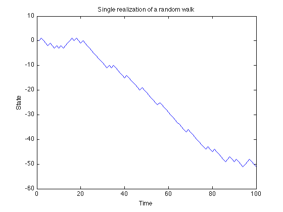
Single realization

To obtain a single realization of a random walk we use the function randomWalk using only two parameters. We set a to be 0.25 and the number of iterations for the random walk is set to 100.

a = 0.25;
x = randomWalk(a, 100);
plot(x);
xlabel('Time');
ylabel('State');
title('Single realization of a random walk');

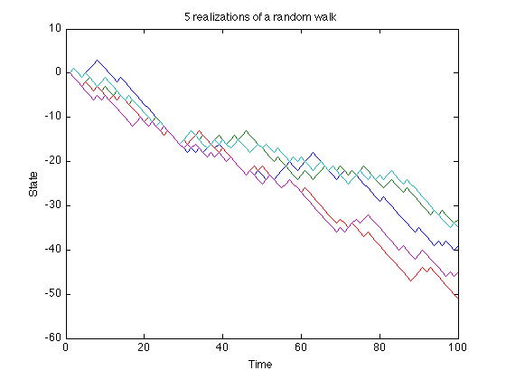
5 realizations

We now use the optional 3rd parameter

x = randomWalk(a, 100, 5);
plot(x);
xlabel('Time');
ylabel('State');
title('5 realizations of a random walk');

Mean Field

We use the function to obtain 10^4 random walks each one with 1000 points. First, we can start the timer to keep track of how much time the computer spends executing the function.

tic;
x = randomWalk(a, 1000, 1e4);

We can know see how long it took to complete the simulations.

seconds = toc;
fprintf(1, 'Time spent in function randomWalk = %g seconds.\n', seconds)

Time spent in function randomWalk = 1.36036 seconds.

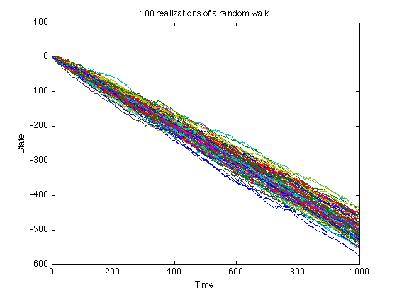
Plot of 100 random walks

plot(x(:, 1:100));
xlabel('Time');
ylabel('State');
title('100 realizations of a random walk');

To compute the average state at each iteration we use the function mean using two arguments. Recall that x is a matrix where each column is a random walk. What we wish to compute is the mean state, that is, we need to find the mean of each row of the matrix. We do so by using mean(matrix, dim). If dim is 2 then mean(x, 2) is a column vector containing the mean value of each row.

m = mean(x, 2);

To compute the standard deviation we can use the std function. The second parameter in std is a flag. This flag is set to 0 in order to compute the non-biased sample std. The 3rd parameter is set to 2 in order to compute the standard deviation along the rows.

s = std(x, 0, 2);

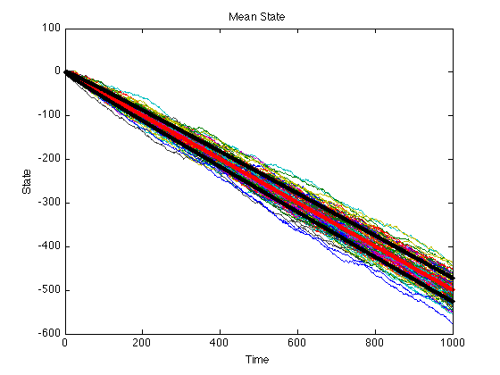
We retain the last plots on the figure by using the command hold on. We then plot the mean and one standard deviation away from the mean. The mean is the red plot and the std lines are the black plots.

hold on;
plot(m, 'r', 'Marker', '.');
plot(m+s, 'Color', [0 0 0], 'Marker', '.');
plot(m-s, 'Color', [0 0 0], 'Marker', '.');
xlabel('Time');
ylabel('State');
title('Mean State');

Note on Color option: To specify a different color you need to change the values on the 1 by 3 matrix. These numbers need to be selected from the unit interval [0, 1]. Each number specifies the value of Red, Green and Blue, in that order (RGB). To obtain the color white, we set all colors to 1. To obtain black, we set them all to 0. To obtain a solid red we can use [1 0 0].

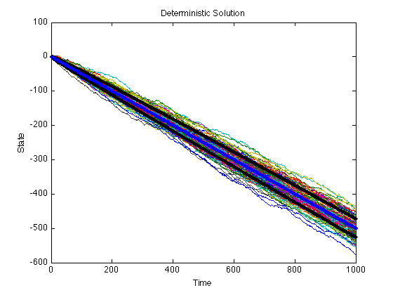
Deterministic Solution

We can compare the mean field with the deterministic solution of the system. We know that the probability of the state increasing by 1 is a and the probability of decreasing is 1 - a. Thus if y denotes the state of the system we can write:

  y(i+1) = +(a) -(1 - a) + y(i)

which tells us that the overall change in the system is:

  y(i+1) - y(i) = 2a - 1

This means that in average the system will have the state:

  y(t) = (2a-1)t

during the t iteration.

The plot of the line y(t) = (2a-1)t is plotted next in blue:

plot((2*a-1)*(1:length(m)), 'Color', 'b', 'Marker', '.');
xlabel('Time');
ylabel('State');
title('Deterministic Solution');

Published with MATLAB® 7.6